In the first case a simple sphere surface is approximated as it changes into a sphere with a radius of twice the original size. In the first few pictures the system samples the initial surface provided by the user and then refines the initial approximation of the surface. The surface is then morphed into a larger sphere using the forces discussed above as well as minor particle addition. The transition from a small to a large sphere is done smoothly in real time. As shown, the final representation of the surface matches the shape provided by the user.
(a)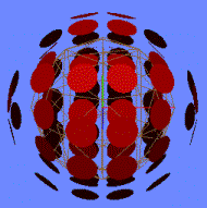 (b)
(b)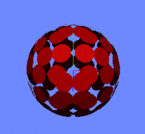
(c)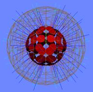 (d)
(d)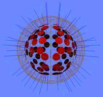 (e)
(e)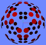
Figure
7: Initial and final representations of a sphere. (a) The
initial sampling is very inaccurate: attraction forces are applied to the
particles to draw them towards the unit sphere. (b) The unit sphere is now
appropriately represented, and is ready to be morphed into another surface. (c)
The sphere is now told to morph into a sphere twice as large. The final surface
is represented with a wireframe mesh, and the net forces on each particle are
shown in blue. (d) Approximately midway through the morph into the larger
sphere. The particles have spread apart but the shape remains spherical. (e)
The end stage of the morphing process. The larger sphere is now visualized.
In the second case a surface created from revolving a sin function around a principle axis is sampled. Even in a more complex surface than that of a sphere, an oriented particle system provides a good visualization. The error between the initial surface as generated with a marching cubes algorithm and the position of the particles in the system is near zero, and the system remains stable in that configuration.
(a)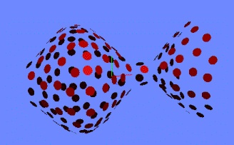
(b)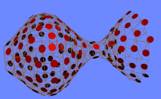
Figure 8: A surface of revolution created with a sine function. (a) The surface shown after initial representation. (b) Particles with surface wire mesh.
The surface from case 2 is then morphed into another surface of revolution created from a sin function with smaller amplitude. Figure 3 shows the surface in varying stages of the morph into the final surface. In the early stages of the morph some particles are being pushed outwards (as they were located inside the new surface) and some are being pushed inwards, while the few particles that happened to be near the final surface undergo mainly rotational changes due to torque forces created by the local gradient. In the final stages of the morph additional particles are added to the surface to create a more representative visualization of the surface.
(a)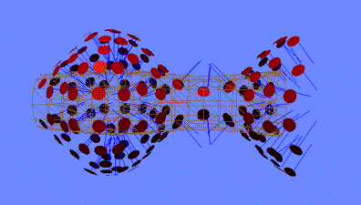
(b) 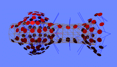
(c)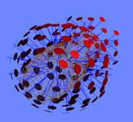 (d)
(d)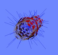
(e)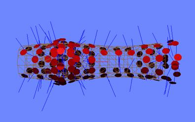 (f)
(f)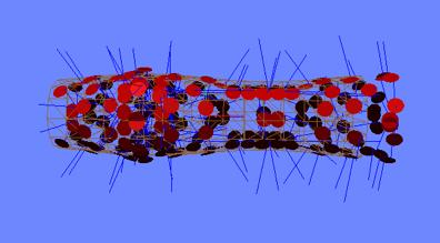
Figure 9: The surface of revolution being morphed into a sine revolution surface with much lower amplitude. (a) Initial surface with final surface drawn in wireframe. (b) An early intermediate morph. Note how the exterior particles are being drawn inwards, while the interior particles are being pushed out. (c) Front view of (b). (d) A near final approximation of the surface. At this point the particles are almost exactly placed on the surface with the forces winding down. (e) Side view of (b). Note the empty region where there were few particles in the initial surface representation. (f) Particles have been added to the surface, filling the empty region.
In
the third case, a surface which consists of two spheres is initially sampled.
These spheres are then moved closer to each other, and finally collide,
creating a topological change in the surface being represented. In the initial
stages of the morph the particles in the upper sphere are moved downwards with
directional forces, as well as some very minor rotational forces (each particle
moves to a slightly different position on the lowered sphere, so has a slightly
different orientation). When the surface changes topologies, several particles
are found to be inside the new surface. These particles are attracted to the
outside using the normal surface attraction and gradient attraction forces. No
user intervention or manipulation of system variables was required to attain
the topological changes required to morph into the final surface.
(a)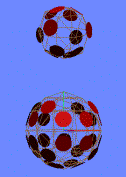 (b)
(b)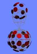 (c)
(c)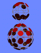 (d)
(d) 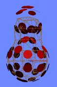 (e)
(e)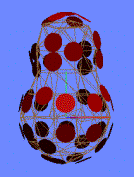 (f)
(f)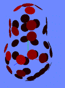
Figure
10: Two spheres are merged together. (a) Initial representation
of the surface. (b) Morphing into the second “key” surface. (c) Near final
stage of morph into second surface. (d) Morphing into final surface. (e) Final
representation of the surface where the two spheres have merged. (f) Final
surface without wireframe model drawn.
In the final case, a sphere with radius of two units is morphed into a cylinder with a radius of one unit. This case requires both topological changes and a significant amount of particle movement. Shown below is a detailed series of screenshots which depict this morph. Of course, justice cannot be done to any kind of animation with a series of pictures. Most of the pictures for this morph do not show the final surface so that a better idea can be gained about how the morphs look. However, in a few samples the target surface is drawn so that the changes can be made more obvious.
(a)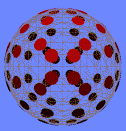 (b)
(b)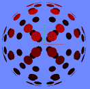 (c)
(c)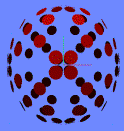
(d) 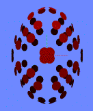 (e)
(e)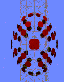 (f)
(f)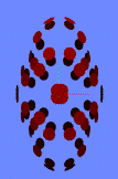
(g)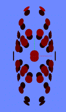 (h)
(h)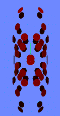 (i)
(i) 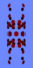
(j)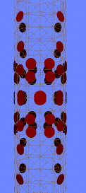 (k)
(k)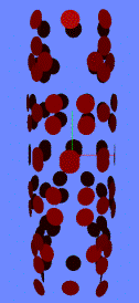 (l)
(l) 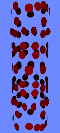
Figure 11: A sphere being morphed into a cylinder. (a)-(b) Initial surface of sphere. (c) Very early stage in the morph. (d)-(i) Intermediate stages in the morph. (j) Final surface approximation when no particle addition is used. (k) Particles added to the final surface approximation. (l) The final surface after the added particles have moved into their final positions.